Complex Wavelets

Notebook

View in Jupyter-Notebook

A quick example to compare different wavelets

import numpy as np
import matplotlib.pyplot as plt

import spkit
print('spkit-version ', spkit.__version__)
import spkit as sp
from spkit.cwt import ScalogramCWT
from spkit.cwt import compare_cwt_example

x,fs = sp.load_data.eegSample_1ch()
t = np.arange(len(x))/fs

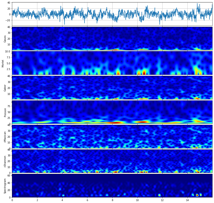
compare_cwt_example(x,t,fs=fs)

---

Gauss wavelet

The Gauss Wavelet function in time and frequency domain are defined as \(\psi(t)\) and \(\psi(f)\) as below;

\[\begin{split}\psi(t) &= e^{-a(t-t_0)^{2}} \cdot e^{-2\pi jf_0(t-t_0)}\\ \psi(f) &= \sqrt{\pi/a}\left( e^{-2\pi jft_0}\cdot e^{-\pi^{2}((f-f_0)^{2})/a}\right)\end{split}\]

where

\[a = \left( \frac{f_0}{Q} \right)^{2}\]

Parameters for a Gauss wavelet:

• f0 - center frequency

• Q - associated with spread of bandwidth, as a = (f0/Q)^2

import numpy as np
import matplotlib.pyplot as plt

import spkit
print('spkit-version ', spkit.__version__)
import spkit as sp
from spkit.cwt import ScalogramCWT

Parameters for a Gauss wavelet:

• f0 - center frequency

• Q - associated with spread of bandwidth, as a = (f0/Q)^2

Plot wavelet functions

fs = 128                                   #sampling frequency
tx = np.linspace(-5,5,fs*10+1)             #time
fx = np.linspace(-fs//2,fs//2,2*len(tx))   #frequency range

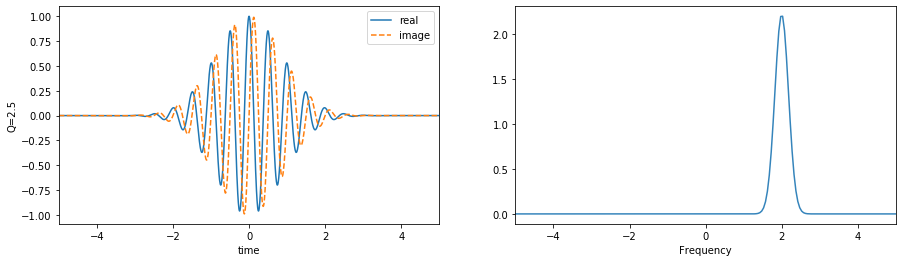
f01 = 2     #np.linspace(0.1,5,2)[:,None]
Q1  = 2.5   #np.linspace(0.1,5,10)[:,None]
wt1,wf1 = sp.cwt.GaussWave(tx,f=fx,f0=f01,Q=Q1)


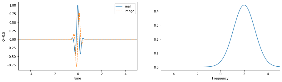
f02 = 2    #np.linspace(0.1,5,2)[:,None]
Q2  = 0.5  #np.linspace(0.1,5,10)[:,None]
wt2,wf2 = sp.cwt.GaussWave(tx,f=fx,f0=f02,Q=Q2)

plt.figure(figsize=(15,4))
plt.subplot(121)
plt.plot(tx,wt1.T.real,label='real')
plt.plot(tx,wt1.T.imag,'--',label='image')
plt.xlim(tx[0],tx[-1])
plt.xlabel('time')
plt.ylabel('Q=2.5')
plt.legend()
plt.subplot(122)
plt.plot(fx,abs(wf1.T), alpha=0.9)
plt.xlim(fx[0],fx[-1])
plt.xlim(-5,5)
plt.xlabel('Frequency')
plt.show()

plt.figure(figsize=(15,4))
plt.subplot(121)
plt.plot(tx,wt2.T.real,label='real')
plt.plot(tx,wt2.T.imag,'--',label='image')
plt.xlim(tx[0],tx[-1])
plt.xlabel('time')
plt.ylabel('Q=0.5')
plt.legend()
plt.subplot(122)
plt.plot(fx,abs(wf2.T), alpha=0.9)
plt.xlim(fx[0],fx[-1])
plt.xlim(-5,5)
plt.xlabel('Frequency')
plt.show()

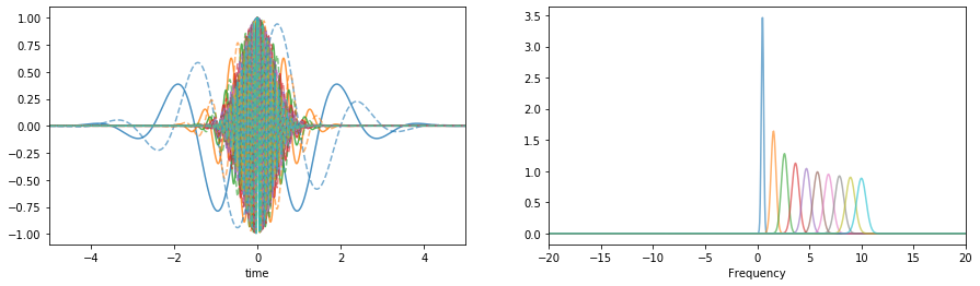
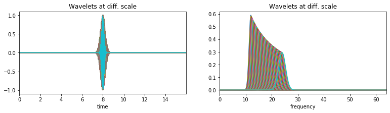
With a range of scale parameters

f0 = np.linspace(0.5,10,10)[:,None]
Q  = np.linspace(1,5,10)[:,None]
#Q  = 1

wt,wf = sp.cwt.GaussWave(tx,f=fx,f0=f0,Q=Q)

plt.figure(figsize=(15,4))
plt.subplot(121)
plt.plot(tx,wt.T.real, alpha=0.8)
plt.plot(tx,wt.T.imag,'--', alpha=0.6)
plt.xlim(tx[0],tx[-1])
plt.xlabel('time')
plt.subplot(122)
plt.plot(fx,abs(wf.T), alpha=0.6)
plt.xlim(fx[0],fx[-1])
plt.xlim(-20,20)
plt.xlabel('Frequency')
plt.show()

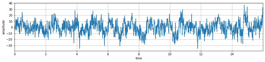
Signal Analysis - EEG

x,fs = sp.load_data.eegSample_1ch()
t = np.arange(len(x))/fs

print('shape ',x.shape, t.shape)

plt.figure(figsize=(15,3))
plt.plot(t,x)
plt.xlabel('time')
plt.ylabel('amplitude')
plt.xlim(t[0],t[-1])
plt.grid()
plt.show()

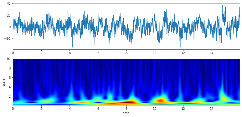
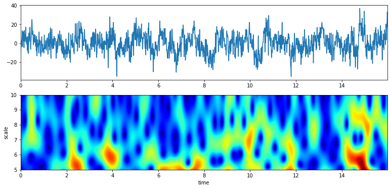
Scalogram with default parameters

## With default setting of f0 and Q # f0 = np.linspace(0.1,10,100) # Q = 0.5

XW,S = ScalogramCWT(x,t,fs=fs,wType='Gauss',PlotPSD=True)

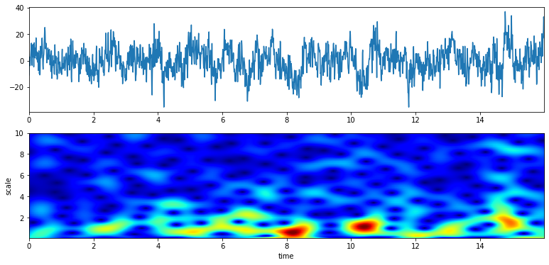
With a range of frequency and Q

# from 0.1 to 10 Hz of analysis range and 100 points

f0 = np.linspace(0.1,10,100)
Q  = np.linspace(0.1,5,100)
XW,S = ScalogramCWT(x,t,fs=fs,wType='Gauss',PlotPSD=True,f0=f0,Q=Q)

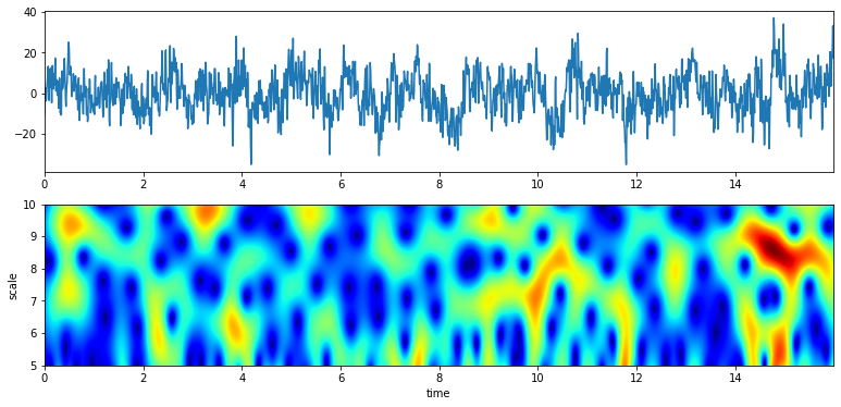
# from 5 to 10 Hz of analysis range and 100 points

f0 = np.linspace(5,10,100)
Q  = np.linspace(1,4,100)
XW,S = ScalogramCWT(x,t,fs=fs,wType='Gauss',PlotPSD=True,f0=f0,Q=Q)

# With constant Q

f0 = np.linspace(5,10,100)
Q  = 2
XW,S = ScalogramCWT(x,t,fs=fs,wType='Gauss',PlotPSD=True,f0=f0,Q=Q)

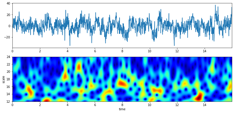
# From 12 to 24 Hz

f0 = np.linspace(12,24,100)
Q  = 4
XW,S = ScalogramCWT(x,t,fs=fs,wType='Gauss',PlotPSD=True,f0=f0,Q=Q)

With a plot of analysis wavelets

f0 = np.linspace(12,24,100)
Q  = 4
XW,S = ScalogramCWT(x,t,fs=fs,wType='Gauss',PlotPSD=True,PlotW=True, f0=f0,Q=Q)

#TODO Speech/Audio Signal

Speech

#TODO

Audio

#TODO

Morlet wavelet

#TODO

The Morlet Wavelet function in time and frequency domain are defined as \(\psi(t)\) and \(\psi(f)\) as below;

\[\begin{split}\psi(t) &= C_{\sigma}\pi^{-0.25} e^{-0.5t^2} \left(e^{j\sigma t}-K_{\sigma} \right)\\ \psi(w) &= C_{\sigma}\pi^{-0.25} \left(e^{-0.5(\sigma-w)^2} -K_{\sigma}e^{-0.5w^2} \right)\end{split}\]

where

\[\begin{split}C_{\sigma} &= \left(1+ e^{-\sigma^{2}} - 2e^{-\frac{3}{4}\sigma^{2}} \right)^{-0.5}\\ K_{\sigma} &=e^{-0.5\sigma^{2}}\\ w &= 2\pi f\end{split}\]

XW,S = ScalogramCWT(x,t,fs=fs,wType='Morlet',PlotPSD=True)

Gabor wavelet

#TODO

The Gabor Wavelet function (technically same as Gaussian) in time and frequency domain are defined as \(\psi(t)\) and \(\psi(f)\) as below;

\[\begin{split}\psi(t) &= e^{-(t-t_0)^2/a^2}e^{-jf_0(t-t_0)}\\ \psi(f) &= e^{-((f-f_0)a)^2}e^{-jt_0(f-f_0)}\end{split}\]

where \(a\) is oscilation rate and \(f_0\) is center frequency

XW,S = ScalogramCWT(x,t,fs=fs,wType='Gabor',PlotPSD=True)

Poisson wavelet

Poisson wavelet is defined by positive integers ($n$), unlike other, and associated with Poisson probability distribution

The Poisson Wavelet function in time and frequency domain are defined as \(\psi(t)\) and \(\psi(f)\) as below;

#Type 1 (n)

\[\begin{split}\psi(t) &= \left(\frac{t-n}{n!}\right)t^{n-1} e^{-t}\\ \psi(w) &= \frac{-jw}{(1+jw)^{n+1}}\end{split}\]

where

Admiddibility const \(C_{\psi} =\frac{1}{n}\) and \(w = 2\pi f\)

XW,S = ScalogramCWT(x,t,fs=fs,wType='Poisson',method = 1,PlotPSD=True)

#Type 2

\[\begin{split}\psi(t) &= \frac{1}{\pi} \frac{1-t^2}{(1+t^2)^2}\\ \psi(t) &= p(t) + \frac{d}{dt}p(t)\\ \psi(w) &= |w|e^{-|w|}\end{split}\]

where

\[\begin{split}p(t) &=\frac{1}{\pi}\frac{1}{1+t^2}\\ w &= 2\pi f\end{split}\]

XW,S = ScalogramCWT(x,t,fs=fs,,wType='Poisson',method = 2,PlotPSD=True)

#Type 3 (n)

\[\begin{split}\psi(t) &= \frac{1}{2\pi}(1-jt)^{-(n+1)}\\ \psi(w) &= \frac{1}{\Gamma{n+1}}w^{n}e^{-w}u(w)\end{split}\]

where

\[\begin{split}\text{unit step function }\quad u(w) &=1 \quad \text{ if $w>=0$ }\quad \text{else } 0\\ w &= 2\pi f\end{split}\]

XW,S = ScalogramCWT(x,t,fs=fs,wType='Poisson',method = 3,PlotPSD=True)

#TODO

Maxican wavelet

Complex Mexican hat wavelet is derived from the conventional Mexican hat wavelet. It is a low-oscillation wavelet which is modulated by a complex exponential function with frequency \(f_0\) Ref..

The Maxican Wavelet function in time and frequency domain are defined as \(\psi(t)\) and \(\psi(f)\) as below;

\[\begin{split}\psi(t) &= \frac{2}{\sqrt{3}} \pi^{-\frac{1}{4}}\left(\sqrt{\pi}(1-t^2)e^{-\frac{1}{2}t^2} - \left(\sqrt{2}jt + \sqrt{\pi}erf\left[\frac{j}{\sqrt{2}}t \right] (1-t^2)e^{-\frac{1}{2}t^2}\right)\right)e^{-2\pi jf_0 t}\\\\ \psi(w) &= 2\sqrt{\frac{2}{3}}\pi^{-1/4}(w-w_0)^2e^{-\frac{1}{2} (w-w_0)^2} \quad \text{ if $w\ge 0$,}\quad \text{ 0 else}\end{split}\]

where \(w = 2\pi f\) and \(w_0 = 2\pi f_0\)

XW,S = ScalogramCWT(x,t,fs=fs,wType='cMaxican',PlotPSD=True)

#TODO

Shannon wavelet

Complex Shannon wavelet is the most simplified wavelet function, exploiting Sinc function by modulating with sinusoidal, which results in an ideal bandpass filter. Real Shannon wavelet is modulated by only a cos function Ref.

The Shannon Wavelet function in time and frequency domain are defined as \(\psi(t)\) and \(\psi(f)\) as below;

\[\begin{split}\psi(t) &= Sinc(t/2) \cdot e^{-2j\pi f_0t}\\ \psi(w) &= \prod \left( \frac{w-w_0}{\pi} \right)\end{split}\]

where

where \(\prod (x) = 1\) if \(x \leq 0.5\), 0 else and \(w = 2\pi f\) and \(w_0 = 2\pi f_0\)

XW,S = ScalogramCWT(x,t,fs=fs,wType='cShannon',PlotPSD=True)

#TODO